Earlier in this chapter we showed how to test for the statistical significance of the Pearson r and that we can construct a confidence interval about the r value. We can also test whether the regression equation is statistically significant and can construct a confidence interval about the slope coefficient (b) from the regression analysis. As it turns out, for bivariate regression the test of the significance of r and the significance of b is redundant. If r is significant, the regression equation is significant. However, we address the process here because it will help you understand the workings of multiple regression, which is addressed in chapter 9.
To test the statistical significance of b and calculate the confidence interval about b, we use a test statistic called t. The t statistic, which is somewhat analogous to a Z score, is examined in more detail in chapter 10, where techniques to examine differences between mean values are introduced. However, the t statistic is useful for more than just comparing means. The t statistic is based on a family of sampling distributions that are similar in shape to the normal distribution, except the tails are thicker than a normal distribution. When sample sizes are small, the t distributions more accurately reflect true probabilities than does the normal distribution.
When we test the statistical significance of b, we are testing whether the slope coefficient is significantly different from zero. (We can also test whether b differs from some hypothesized value other than zero, but this is rarely done in kinesiology.) The statistical hypotheses for a two-tailed test are as follows:
H0: b = 0
H1: b ≠ 0.
The degrees of freedom for the test are n − 2. The test statistic t for this analysis is calculated as (Lewis-Beck, 1980):
 (8.14)
where b is the slope coefficient and SEb is the standard error of b. We calculate the standard error of b as
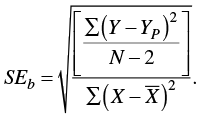 (8.15)
Notice what this equation is telling us. Inside the radical, the numerator is reflecting how much error is in the predictions, because we are adding up the squared differences between the actual Y scores and the predicted Y scores (once again a sums of squares calculation) and dividing it by a degrees of freedom term (a sort of mean square because we are taking a sum and dividing it by a degrees of freedom term). The denominator is the sums of squares for X, the independent variable. The better the prediction of Y based on X, the smaller will be the standard error of b. The smaller the standard error of b, the larger will be the t statistic, all else being equal. The larger the t statistic, the less tenable is the null hypothesis.
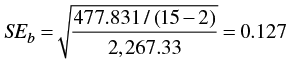
Fortunately, most of the work in this calculation has been done already in table 8.3. Substituting the appropriate terms into equation 8.15, we get
To calculate t, we substitute the appropriate values into equation 8.14 so that
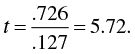
To determine the statistical significance of t, we can use table A.3a in the appendix. To be statistically significant at a two-tailed α = .05 and with df = 13, the calculated t must be ≥ 2.16. Because 5.71 > 2.16, we can reject H0 and conclude that the number of push-ups is a significant predictor of isometric time to failure. Recall that t is analogous to Z but is used in cases of small sample sizes. Table 7.1 on page 72 shows that a Z score of 1.96 corresponds with a 95% LOC (two-tailed). With 13 df, the 95% LOC (two-tailed) corresponds to a t value of 2.16. The t value associated with the 95% LOC value (2.16) is larger than the Z value associated with the 95% LOC value, which is reflective of the thicker tails of the t distribution relative to the normal distribution. Examine table A.3a for the two-tailed data under the .05 α level. Notice that as the degrees of freedom get larger, the tabled values for t get smaller so that at df = ∞, the values for t and Z are equal. That is, as the degrees of freedom increase, the t distribution approaches a normal distribution. (One can consider the normal distribution as just a special case of the t distribution with infinite degrees of freedom.)
We also use the t distribution to calculate a confidence interval about the slope coefficient. The confidence interval is calculated as
 (8.16)
where t is the critical t value from table A.3a for a given α and degrees of freedom. For the push-up data, the t value we need (95% LOC, df = 13) is once again 2.16. Previously, we determined that b = .726 and SEb = 0.127. Therefore, the 95% CI for the push-up data is
.726 ± (2.16)(0.127) = 0.45 to 1.00.
In a journal, we might report this as b = 0.726 seconds per push-up, 95% CI = 0.45, 1.00. Thus, we are 95% confident that the population slope lies somewhere from 0.45 and 1.00 seconds per push-up. Notice that zero is not inside the 95% CI, which means that the slope is statistically significant (p < .05).
In practice, these calculations are rarely performed by hand. They are too cumbersome and it is easy to make arithmetic errors. In addition, at each step rounding error will occur. Statistical software performs these calculations faster and more accurately. Plus, statistical software will generate actual p values that are more precise than those generated from looking values up in a table and reporting, for example, p < .05. Nonetheless, seeing where the numbers come from is useful in developing an understanding of how these tests work.
Sample Size
Ideally, the sample size of a study using correlation and bivariate regression should be determined before the start of the study. Free and easy to use software known as G*Power is available to perform these calculations. G*Power can be downloaded from www.gpower.hhu.de/en.html, and Faul and colleagues (2009) have described how to use the software for sample size calculations with correlation and bivariate regression studies. The primary decisions an investigator must make in this situation are defining the smallest effect that would be of interest and deciding what level of statistical power is desired. For example, assume we determine that the smallest correlation of interest between number of push-ups and time to failure (see table 8.3) is .30. That is, we decide that any correlation less than .30 is too small to be of interest. In addition, we choose a power level of 80% (or 0.80). From G*Power, if we set the correlation to .30 and set α to .05 and power = 0.80, we would need to test 84 subjects. Instead, if we set the smallest correlation of interest to .40 and left the α at .05 and power at 0.80, then only 46 subjects would be necessary. In contrast, if we left the minimal interest to be r = 0.30 and α = .05 but increased the desired power to 0.90, we would need to test 112 subjects.